Conditional Formatting Can Slow Down Your Excel Spreadsheet: Try This Little Known Hack

How to Improve the Speed of Your Conditional Formatting - and a Little Known Trick

Conditional formatting in Excel is a useful tool for many tasks. To name a few examples, you can use it to identify values in certain ranges, particularly high or low values, duplicates, outliers or create heatmaps or data bars. Advanced users also take advantage of conditional formatting to build Gantt charts or calendar-like applications in Excel.

But especially in the later cases or when dealing with large datasets, complex conditional formatting rules can drastically slow down your spreadsheet and seriously compromise your user experience. There are a few common rules to reduce this slow down effect on your workbook, which we will have a short look on.

And then, we will present a simple, but little used trick to cut the refresh time for your conditional formatting more than in half (which we will measure using a VBA timer), without having to cut back on any functionality at all.

Speeding Up Your Conditional Formatting – Some Common Tips

Before we had on, let’s first have a short glace at common knowledge and tips to keep your conditional formatting in Excel fast.

• Keep the amount of data with conditional formatting short: This one is obvious, but the more data you want to highlight with conditional formatting, the more you will impair the speed of your worksheet. If you want to create a Gantt chart or calendar, do you really need 365 days at once? Do you need a granularity of one day? Would a week be enough as well?
• Avoid redundancy and overcomplication: Check your rules after you are done. Do you have redundant rules? Rules that are no longer necessary? Clean up.
• Simple rules: Keep your rules, but also your formulas (if you need to use a formula condition for the rule) simple. Carefully strategizing your calculations (which might include to put some of your calculations in for example a helper column or the cell to evaluate) can reduce the workload Excel has to calculate for each rule).
• Slow or volatile functions: Speaking of formulas and functions. Avoid volatile functions at (almost) all costs (not just in conditional formatting). These include CELL, INDIRECT, INFO, NOW, OFFSET, RAND, RANDARRAY, RANDBETWEEN and TODAY. Also, user defined functions (UDF), meaning those programmed in VBA by yourself, should only be used with caution.
• Avoid fragmentation: A single rule for a large set of data can be fast then several rules for the same number of cells. Be careful not to fragmentate existing rules when you add or remove columns or rows or when copy/cut and pasting cells and ranges.
• Manual mode: While often not desirable, when working with large datasets, putting the calculation mode into “manual” can ease working on your data set.
• The screen size: Yes, even the size and resolution of your screen will have significant impact on the time. The example we show below will take almost 3 times as much time to update on a 3840x2160 screen, compared to a 1920x1080 screen.
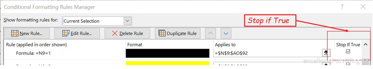
• Use “Stop-if-true” whenever possible: In the conditional formatting rules manager, you will find the option to “stop-if-true” on the right side. In most cases, there are only benefits to put your checkmark here. Excel will evaluate your rules from top to bottom. If the top rule is true, there is typically no need to continue with the evaluation of the rules below and Excel can finish the evaluation of further rules for the cell.

The last tip can be used strategically to speed up complex conditional formatting rules as you will see in the next chapter.

A Little Known, Powerful Hack – Leverage the Stop-If-True Condition to Your Advantage

As already mentioned in the last section, you will find a “stop-if-true” checkmark for every rule in the conditional formatting rules manager. Excel evaluates the rules from the top to the bottom of the list. If one rule is true, Excel will stop evaluating the rules lower down in the list. It is very reasonable to have this mark (almost) always checked.

But, for some applications, like Gantt charts or calendars that are set up with conditional formatting, we can even leverage this opportunity further to our advantage.

Let’s have a look at this calendar, that we have set up for a client.

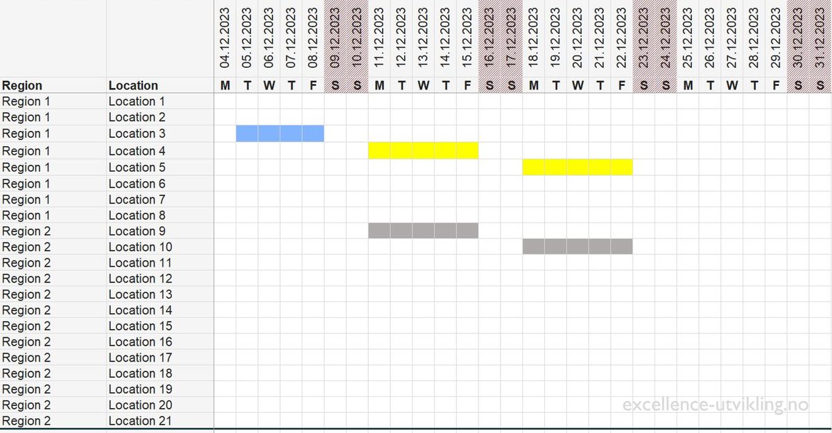
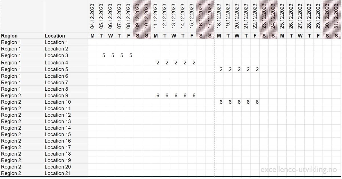
The client has over 80 production locations and 13 resources that they move between these locations to perform certain periodic maintenance tasks. The calendar will lookup the location and date in an Excel table in the background and eventually display the ID of the maintenance resource in the cell, so we can visualize it with condtional formatting.

How does this work? While it is not necessary to go deep into the involved formulas, each cell in the calendar range will look up in a table in the background to check if a resource ID is assigned to the current date and location. If that is the case, the ID of the resource will be populated to the cell. Without conditional formatting, this looks like the following:

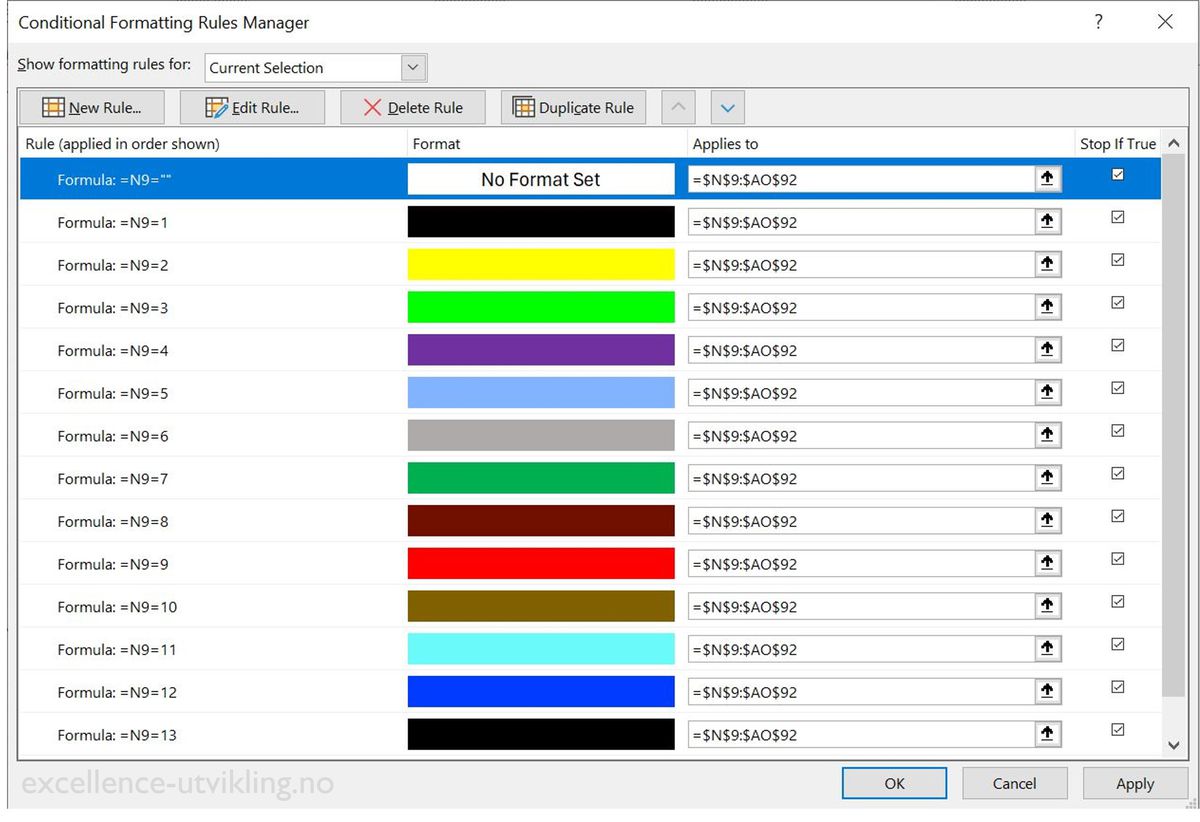
Since the client has 13 resources, we need 13 rules to highlight each resource with an assigned colour (on a side note: the client has a VBA form tool to add new or remove resources, change their colours, do modifications, and so on). The list of rules is therefore long:

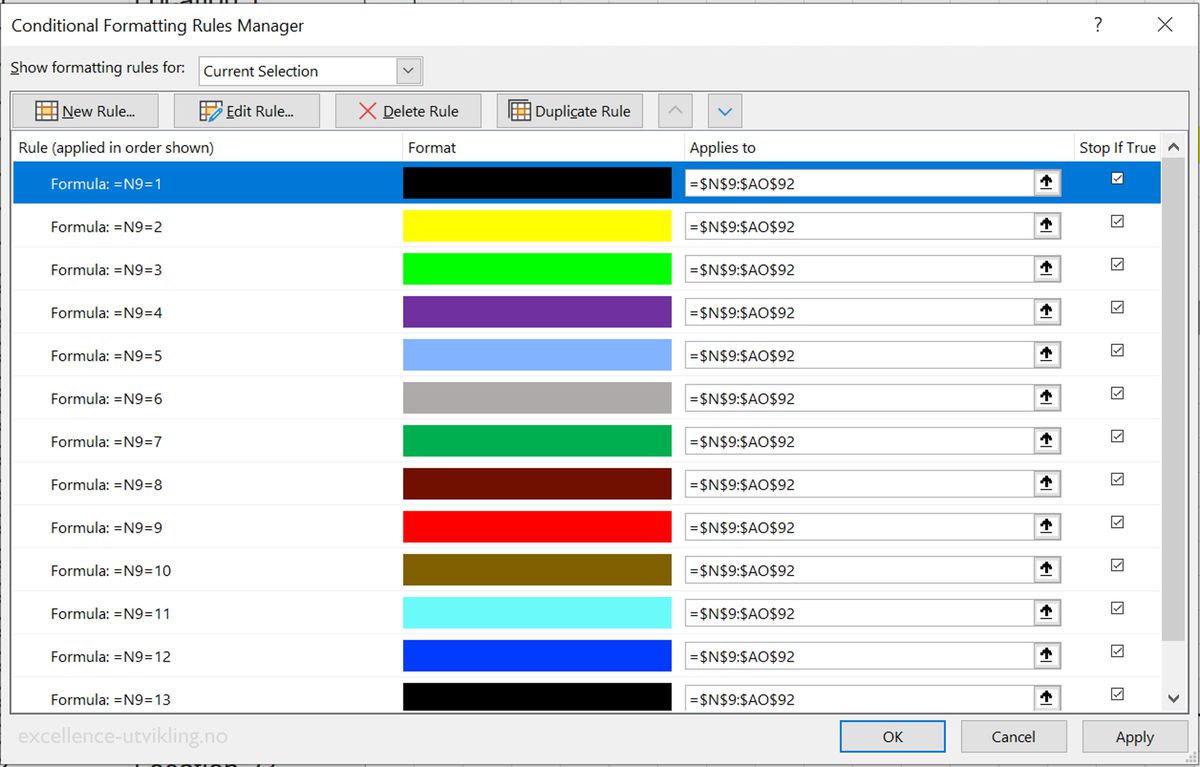
If you remember what we said above, Excel will evaluate all 13 rules until one of them is true, you realize that this will take a long time. At the same time, you might have recognized that the range in the image shows 588 cells – where only a mere 24 contain a number (the actual calendar is even larger).

So, there is no point that Excel needs to evaluate 588 times 13 rules for this (excerpt of a) calendar.

The solution is simple but extremely effective:

We can simply add a rule ahead of the other rules, with no formatting at all, but the stop-if-true condition checked. This rule will simply check if there is a number at all in the cell. If this is not the case, there is no point in evaluating the other 13 rules at all. This way, we can reduce the number of steps to evaluate from more than 7 000 to less then 700 in this little excerpt!

This is, what it looks like in the conditional formatting manager in Excel:

Whenever you are dealing with a large set of rules, where only a few cells should be highlighted, you might consider if an extra rule might be able to speed up your spreadsheet. This might be useful when you have empty cells, text cells, values that are far out of range and so on that do not need any more detailed evaluation. Be creative to find a solution for your specific challenge.

How Much Faster is the Spreadsheet Using This Hack?

Let’s take the time for the update of this calendar. For that purpose, I have written some simple VBA code. You do not necessarily need to understand what happens here. Just in few words: We take the start time first, then we will change the value of cell F3, which will trigger an update of the conditional formatting through some formulas. This is done 10 times to be more accurate and reproducible. Then we take the time again and measure the time passed.

Sub MeasureCalculationTime()
' ----------------------------------------------------------------
' Purpose: Measures the time taken to execute a loop that changes the value of a specific cell to trigger conditional formatting recalculations.
' Author: Michael Markus Wycisk / Excellence Utvikling AS
' Created Date: 04.05.2024
' Change log:
' ----------------------------------------------------------------
    Dim dblStartTime As Double, dblEndTime As Double, dblTimeDifference As Double
    Dim lLoop As Long

    'Capture the Start Time
    dblStartTime = Timer * 1000

    'Force a change in the conditional formatting by changing cell F3
    For lLoop = 1 To 10
        wsCalender.Range("F3").Value = 1
        wsCalender.Range("F3").Value = 2
    Next lLoop

    'Capture the End Time
    dblEndTime = Timer * 1000

    'Calculate and display the passed time
    dblTimeDifference = dblEndTime - dblStartTime
    Debug.Print "Time taken for calculation: " & dblTimeDifference & " ms"
End Sub

So, what is the result. The calendar range stretches from N9 to AO92. That makes it 2 352 cells with 13 rules to evaluate each. Without our hack (the rule checking for the empty cell that stops further evaluation, the result for 10 loops is:

Time taken for calculation: 1578,125 ms

Once we add our new rule that stops the evaluation for all empty cells early, we cut the time down to:

Time taken for calculation: 542,96875 ms

So, we have been able to reduce the time consumption by more then 66%! Important to remember: This is taken from a real-world example delivered to one of our clients. It has to be taken into account that a lot of the remaining 543 ms is the time necessary to evaluate the look up functions towards the data table in the background. These were strictly necessary to fulfil the clients’ requirements. If we had isolated the issue solely to the conditional formatting, the timesaving might have been even higher, likely surpassing 90%.

Partnering for Success: Your Excel Consultant

At Excellence Utvikling AS, we understand the importance of good user experience and the application of best practice techniques when setting up Excel spreadsheets, models and macros for our clients. We will never compromise on quality when we work together with you to solve your challenges.

Our Excel consulting services cover a wide range of services, beyond the design of calendars, Gantt charts or resource planning tools like the one used in this article. Whether it's designing business templates, creating powerful and timesaving Excel automations or tackling complex data challenges, our goal is to enable you to make the most out of Excel.

If you're ready to unlock the full potential of Excel in your business, don't hesitate to reach out. We're here to guide you through every step of the process, and we're excited to partner with you to achieve your business goals.